Being organized and creating consistent configurations is a great virtue in the Networking / SDN / Cloud and computing field.  ACI is no exception to that rule.  Haphazard, Inconsistent and thoughtless configurations will increase your work and complexity/understanding of your infrastructure once your  Fabric grows.  In addition it will make it more prone to failures when scaling out.

One often overlooked item is an understanding of TCAM utilization in ACI. In this article,  I will discuss TCAM usage and give you tips on how to optimize and watch it.  It is assumed that you are already familiar with ACI, especially contracts and how to use contracts.  I highly suggest you read / bookmark the following link: Everything you want to know about ACI Contracts 

TCAM is short for Ternary CAM.  TCAM is a very precious resource and if you exhaust it you are done for.  TCAMs ability to perform bulk searches of the entire content with matches based on 0’s, 1’s and * (wild card)  makes it an ideal candidate for high speed constantly updating (real-time) /searchable direct access database (without involving the OS).  That is why it is extensively used in high performance networking equipment. 

However,  TCAM is expensive to build, consumes a lot of power and generates a high level of heat that needs to be dissipated.   For that reason,  TCAM capacity is not unlimited and you need to understand how TCAM is utilized in ACI to make sure to optimize your fabric so you don’t run out of TCAM as your Fabric grows.

The TCAM I am referring to when mentioning ACI TCAM is the TCAM on the ACI leaves.  Every Leaf Node in the ACI Fabric has it’s own TCAM.  That is why you need to look at TCAM utilization on a per leaf basis.  There is no concept of Global TCAM for the entire fabric.  In this article I will only discuss Gen 2 leaves and higher and will work with ACI Release 5.1.(2e)

On the APIC UI you could go to Operations/Leaf Capacity and get a bird’s eye view of your number of rules in Policy CAM.  From that you can get an estimate on which leaves are on the edge.  For instance in the magnified view below, Leaf-102 shows to have 88 rules out of a total capacity of  65K rules, so we are doing good.  However this is a rudimentary look and you need to get a bit deeper into it.

So, you may be tempted to think that the 64K entry space in the above figure is the TCAM.  Actually it is not.

That 64K is actually the Policy CAM carved up capacity of a static RAM (SRAM), which works in conjunction with the fixed TCAM size of 8K.   The 64K space is called the Policy CAM whereas the real TCAM of 8K is called the APP CAM or more often called the Overflow TCAM.

The  SRAM can be changed to carve up different  / reserved capacity for Policy CAM and other functions.  As an example on a border Leaf you might want to hold more LPM (Longest Prefix Match ) entries, because you might have more routing prefixes.  If you chose the “High LPM” profile, for the border leaves (let’s assume FX2 leaf), your LPM capacity would increase to 128K at the cost of Policy CAM of 8000.  The default Dual Stack Profile would give you 20K LPM and 64K Policy CAM.   You can see the different forwarding scale profiles for ACI 5.1.1 release at the following link:   Forwarding Scale Profiles

Forwarding Scale Profiles can be changed by the following 3 step process.

1. Define the ACI Forwarding scale (from Fabric/Access Policies/Policies/Switch.  As an example HighLPMBorderLeaf
2. Attach the policy the leaf using a defined Policy Group ( from Fabric / Access Policies/Leaf Switches Profile ).  The Policy Group in turn should reference to the ACI Forwarding  Scale you defined in step 1.
3. Reload the switch/switches where you changed the Forwarding Scale to a new profile.

The 64K Policy CAM  (SRAM) for all practical purposes works as an extension to the 8K Overflow TCAM (Real TCAM).  It does parallel lookup in the same instance in time.  This is done with the aid of a hash table.   The hash is derived from numerous fields in the contract, such as Source EPG, Destination EPG, Protocol, L4 ports, TCP fields, etc, etc.

The Policy CAM can only install entries with similar hash.  As such with the capability of manipulating the Policy CAM  with Forwarding Profiles  and also because it has more capacity than the Overflow TCAM, it turns out to be more versatile and for that reason, Policy CAM is prioritized over Overflow TCAM.  The algorithms and heuristics will try to save Overflow TCAM space by using Policy CAM hashing for the largest rule set (in entries) and the smaller rule sets in Overflow TCAM for a particular set of EPGs.

The main purpose for Overflow TCAM as it turns out is to handle outlining policy rules that cannot exist in Policy CAM due to hash collision.  Hence the name overflow TCAM.  As an example, let’s say you want to use L4 port ranges in your contract between EPGs.  Policy CAM can handle a single port range efficiently and up to 4 different port ranges can be handled efficiently.  After 4, the limited resource in Overflow TCAM is used to store the entries.  * Hint:  in a contract between EPGs, don’t use more than 4 sets of port ranges.  It’s best to keep it at 3.

A Practical Approach:

Now that we’ve spoken about the theory, you might say “Great !  now what does all this mean and what do I have to do to make sure that I don’t run  into TCAM exhaustion ? “

Let’s look at this from a practical approach which might start making more sense.  As we go along I’ll point out Good Practices (based on situation), common mistakes, etc, etc.   

At the end,  I’ll also summarize all the commands I will use in 1 place, so it’s easy to use them.

1.  Forwarding Scale Profiles for dedicated Border Leaves: We’ve already discussed 1 possibility for dedicated border leaves.  If you have a production Fabric, you should invest in dedicated border leaves and based on your  situation choose to change the Forwarding Scale Profile for the border leaves.    If border leaves are dedicated, they probably won’t have many endpoints and no user EPGs, hence they might not require that much Policy CAM space, but might need more space for holding LPM entries.   You can see the different forwarding scale profiles for ACI 5.1.1 release at the following link:   Forwarding Scale Profiles.  One more consideration is what sort of hardware should you use for your border leaves.  The link also shows you the Forwarding Scale Profiles for EX and FX2 leaves as compared to GX  and FX leaves.

1.  

• • To see the LPM / TCAM entries on Border leaf use the command:

    vsh_lc -c "show platform internal hal l3 routingthresholds"   # use on border Leaf

2. Distribute your  Application EPGs across Leaves:  TCAM utilization is on a per Leaf basis.   The formulae for calculating number of rules (each rule taking up a TCAM entry),  is:   number of Consumer EPGs * number of Provider EPGs * number of rules per EPG.  If your application had 20 EPGs with full mesh of contracts with 2 rules you would have 20 * 19 * 2 = 760 rules using 760 entries in TCAM.  If all the 20 EPGs were on 1 leaf, then you would add  all 760 entries on the TCAM of that leaf.   If the EPGs were distributed across leaves, then the TCAM entries would be distributed across leaves.

3. Be Familiar on how to look at contracts from cli:   You don’t need to do this at this time.  I’m just including this to give you some useful commands to check with when looking at contracts.

Let’s take an example on how to do this with a very simplistic example:

Let’s say I need to bring up 2 EPGs for a APP in a new VRF. 

item 1:  find out the scope for the EPG.   You can do this from GUI ofcourse, but let’s do everything from CLI. 
From APIC, ssh session do:

"moquery -c fvctx" | grep SM-VRF -A 10    #  my VRF name is SM-VRF

item 2:  find out the pcTags for the EPGs
for this I will use the command:

moquery -c fvEPg | grep L30 -B 5 -A 8  #  do this on the Leaf where your EPG is,  I'm grepping on L30 because my epg names start with L30

item 3:    Check the rules that are in that VRF.  Use the scope ID for it.
At this time I have not added any contracts, so, the only rules will be default implicit rules that is in every EPG.
Use the command:

show zoning-rule scope 2588673  # do this on the leaf.  2588673 is the scope of the VRF we got in an earlier step

Note that the pcTag Ids are all in the ranges that are system default at this point.  For your reference here is a list of them:

The pcTags can have either a localor globalscope: 

• System Reserved pcTag– This pcTag is used for system internal rules (1-15).
• Globally scoped pcTag– This pcTag is used for shared service (16-16385).
  Locally scoped pcTag– This pcTag is locally used per VRF (range from 16386-65535).

 

item 4:    Another useful command to see what rules are between 2 EPGs, you can  Use the command:

show zoning-rule src-epg 49153 dst-epg 32770 # do this on Leaf

Note:    In this case, I don’t have any contracts between the EPGs so the output does not show any entries.

item 5:     If you did have contracts you would get output from the previous command.  That output would show a Pririoty value for each rule.   The lower the priority, the earlier it will be on the list.  If you had multiple rules, you would see each line with a priority (think access-list).   Sometimes 2 different lines might have the same priority.  In that case, you would need to check the hardware index of the rules.   You would use the rule ID’s of the line items to check for this.   The lower hw_index has priority.
Command to use:

vsh_lc -c "show system internal aclqos zoning 4175"  # do this on leaf.  here 4175 is a rule ID  

item 6:   If you wanted to see more details on any filter, let’s say one of our implicit filters you saw above  “implarp”, you could use the command:

show zoning-filter filter implarp  # do this on Leaf

item 7:   In case you wanted to see if any traffic is hitting any rule, you can use the command:

show system internal policy-mgr stats | grep 2588673  # do this on leaf.  2588673 is the scope ID of the VRF

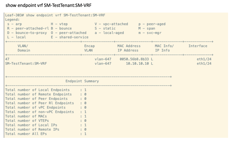
item 8:   Please realize that even if you have static bindings or VMM bindings but no endpoints on those EPGs (maybe VMs were never fired up),  the contract rules will not get applied (unless you did a deployment/resolution  to be immediate/immediate).   In ACI unless a resource is needed, it does not apply it.  This is how ACI scales so well.  To check if endpoints are available on a VRF you can use the following basic command:

show endpoint vrf SM-TestTenant:SM-VRF  # do this on the leaf where you did your binding.  

If you wanted to get more granular and see if the EPG has endpoints (instead of the VRF), you can use the command:

moquery -c fvLEpP -f 'fv.LEpP.polInstrumented=="yes"' | grep -A 12 -B 5  L303  # do this on Leaf.  I'm grepping on L303 because my EPG name has L303

4. Baseline your TCAM utilization:   Before bringing up a new app, baseline your TCAM utilization.  Remember, that you cannot run out of either Policy CAM or Overflow TCAM.   If you are at 70% utilization on either of these CAMS, you probably need to slow down bringing up more EPGs  (meaning doing VMM or static bindings) on those leaves that have that 70% utilization or more (the number is subjective, but I would start watching very close).   Use the following command:
   

   vsh_lc -c "show platform internal hal health-stats" | grep _count  # do this on Leafs where your EPGs will have endpoints

To get details on the Hash Entries , you can use the command:

vsh_lc -c "show platform internal hal policy stats region all"  # do this on Leaf where your EPG endpoints are

5. Use vzAny Contracts when possible:   In some situations where you many need a full mesh of contracts or close to it,  using vzAny contracts is a great option. Not only does the configuration becime simpler, it also saves tremendously on CAM utilization.  The reason for this is the entire group of EPGs is treated as one entry.  Let’s look at this from the figures below.
   

   Example 1:
   Here we have 5 EPGs. EPG-E is provider and all others are consumer to it. If you did a normal mesh of contracts you would use 8 rules. If you did vzAny contract you would use 2 rules.

Example 2:
In this case we have 4 EPGs and everyone is a provider/consumer.  There are 2 rules per EPG.  In this case using normal full mesh of contracts would consume 24 entries, whereas vzAny would only consume 2.

6. Use Contract Filter Compression if you have a large number of rules:  When you attach a filter to the subject line of a contract, you have the option to specify policy compression for the filter entry.   Turning on compression, cuts the CAM utilization value in half. 

* Note that it does not decrease the number of rules, but it does decrease the amount of Policy CAM / Overflow TCAM consumed in half.    The downside of configuring contract compression is that you loose statistics on the entry.  Also,  some kind of filters cannot be compressed for e.g. filters containging priority, DSCP mark Directivies.   In addition vzAny contract filters cannot be compressed.   When enabling contract compression you will get a warning popup in APIC UI.

In the below example I added a contract with only 1 rule (allow ssh).  With the default Disalbed Policy Compression, both my Policy CAM and the Overflow TCAM increased by 2.

Next, I went ahead and modified the contract and changed the ssh filter on the contract to be Compressed Policy.  

Note that both the Policy CAM and Overflow TCAM utilization got cut in half.

7. Understand the implication of putting contracts rule by rule:   When contracts are entered filter at a time (instead of range of ports), both the Policy CAM and the Overflow TCAM increase linearly.  This works fine in the case of smaller setup or taking a Network Centric approach.  However even with contract compression,  your maximum rule by rule entry would be limited by the overflow TCAM which is 8K only.  To overcome this problem the mechanism is that 2K hash banks will be used freeing up space in the 8K oveflow table. The hash bank comes from the Static RAM regions.  You shoud never have a situation where the Overflow TCAM is full and the Policy CAM has space left with single line Contract Filter entries.  Thus for single line Contract entries, monitoring the Policy CAM for utilization is good enough.   The use of the hash banks can be viewed from the output of the command:
   vsh_lc -c “show platform internal hal policy stats region all” 
   In the below example I’ve taken the last state of the output of (4) where I added a SSH contract.  I then added 5 more contract filters 1 at a time (all policy compressed).  In each step of the way, I checked the CAM utilization and both Policy CAM and Overflow TCAM kept increasing linearly.  At the end for adding 6 indivudual entries I ended up with Policy CAM and Overflow TCAM to increment by 6 entries each.

Next, I want to see what happens if I added a large number of individual Contract Filters.  Based on the Scalability Guide for APIC 5.1.1 release, the verified scalabilty for Filters is 10,000.    I decided to go over that 10,000 number and used Postman Runner to create and add 12,000 individual filters (with compression enabled) to the contract.   I first deleted the older filters.  It took a while to push those filters to the contract through Postman Runner, and while the script was running, I checked the CAM memory many times.   I could see the Hash Banks getting created and entries moved to the Policy CAM, thus constantly freeing up the Overflow TCAM so it does not get exhausted.   At the end,  all the 12,000 entries got pushed to Policy CAM and the Overflow TCAM utilization only increased by 884, leaving ample capacity in Overflow TCAM.   You will also notice that the max_policy_count for Policy CAM decreased by 10K.  This is expected and by design. This 10K is used to create an indirect association between policies and TCAM entries via Policy Group.  This 10K is carved out of the main policy-cam Table.  The final state of the CAM is shown below. 

Below you can see the output of: vsh_lc -c “platform internal hal policy stats region all” .   This shows you that 7 Hash Banks are used.  Also notice the 844 TCAM entries which matches with Figure 20A.

1. 8. Understanding the implication of configuring contracts with range of ports:  In most large setups, especially for Application Centric sort of topologies it will be necessary to use range of ports for filters, rather than adding 1 at a time contract filters. 
      1. We’ve already discussed earlier in this article that you should limit your port ranges on any contract filter to be no more than set of 3 (between any 2 EPGs).   That is because after 4 those entries will stay in Overflow TCAM which is a precious resource.  If you keep adding more and more Contract Filter Ranges, you will have a situation where the Oveflow TCAM starts filling up and not being able to move the entries to the Policy CAM.  Now you can have a situation where the Oveflow TCAM gets exhausted and the Policy CAM still has capacity.   Thus if you are using contract filter port ranges, you should monitor your Overflow TCAM to see how much capacity is left.  If you were just monitoring Policy CAM in this case and you did not follow the rule of keeping the contract filter port ranges to be no more than 3 (between EPG pairs), you would not be aware that your Overflow TCAM is filling up.  You would soon be headed towards an unpleasant surprise. 
      2. When you configure port ranges, it’s best to have large port ranges to get maximum bang for the buck.  What you are aiming for is that the large port ranges gets pushed to Policy CAM and not the small ones.   For that reason,  it’s good practice to not do port ranges for range of ports of 10 or fewer.   Make them individual entries instead.
      3. The next item that I wanted to point out is that when range based entries are pushed in Oveflow TCAM they might expand in multiple blocks consuming many entries.  The most efficient way of handling this if possible is to configure the ranges of ports in bit boundaries.  An easy approach is to do this is to configure port blocks at the start of a  multiple of 16 and end before the start of some other multiple of 16.
         As an example, let’s say that I wanted to configure a range of tcp port 100 to 109.  Let’s see what happens:

You will notice that both the Policy CAM and Overflow TCAM increased by a value of 10 each.  That’s not very good. 
Now, let’s try to configure the port ranges in the bit boundary.   Looking at multiples of 16 we have: 16*6 = 96, 16*7 = 112.   Thus the bit boundary will be 96 – 111 which is inclusive of the ports we wanted, i.e 100 – 109.   Let’s see what happens now.

You will notice that both the Policy CAM and Overflow TCAM increased by a value of 1 each.  This is clearly much more efficient.  Ofcourse, this might not suit your purpose as some extra ports have now been enabled, but this is something to take note of.
In a similar fashion,  even if you configured huge port ranges, but did it in bit boundaries, you will notice that the CAM utilization is very efficient.  As an example,  16*3 =48, 16*3500 = 56000.  If we configured port range 48 to 55999, that would fall in the bit boundary.  Trying to configure a contract with filter (policy-compression enabled), we will see that only 1 Policy CAM is used and 16 Overflow TCAM is used for this huge range of 55,951 tcp ports.  As a matter of practicality, if you had to open up that many ports, you might as well do IP Unspecified Filter with compression.  That will just increase Policy CAM and Overflow TCAM by value of 1.

9. Avoid a common mistake that many folks often do:   Often times,  customers desire to change from Network Centric to Application Centric mode.   To do this they have to have a good understanding of their applications, including the tcp/udp ports that they need to open up between application tiers.   To get this information customers often use some sort of ADM (Application Dependency Mapping ) Tool, for instance Tetration.  They then try to take the output that the Tetration engineer gives them and try to feed it directly into ACI Contract EPGs.   More often than not, this lands them up in a disastrous situation.   The reason, is that the Tetration or other ADM outputs given to the ACI team are not optimally presented, even if they are correct.  Subset of Port Ranges between application tiers are often times duplicated in different contracts  or in the same contract in different port ranges that go between sets of EPGs.  There are 2 downsides of just taking this kind of raw input and deriving ACI contracts out of this. 
   
   1. You use up Policy Cam/Overflow TCAM entries unnecessarily leading to leaves running out of TCAM space and causing an outage.
   2. Your configuration is disorganized causing you unintended results when you try to modify.  As an example, lets say that port 80 is enabled in multiple contracts between a group of EPGs.  You want to modify the contracts to not allow this any more.   When you have so many entries in contracts, it’s hard to spot that you have port 80 allowed in multiple Filter Ranges in that contract or maybe even a different contract that happens to go between those sets of EPGs.  You may spot it in one or two contracts  with port range that has 80 included and delete those entries, however it may turn out that there are other contracts / Port Ranges that have that entry included between those EPGs.  The end rusult is you thought you just disabled port 80 between the sets of EPGs, but in reality you did not.

Let me show you a simplistic example of such a configuration. I say simplistic, because it’s very easy to spot here, but when you have tons of output that Tetration gives you such an overlap will be hard to catch.
Let’s say Tetration gives you  2 port ranges that you need to configure between Publisher Tier and Mqueue Tier components of your applications.  There are multiple MQ tier host clusters and each are listening to differnent ports.
Out of the many port ranges given by the raw output:
Three of the port range entries show:
Consumer -> Provider
Pub  tcp 160-199  MQ
Pub  tcp 185-207  MQ
Pub tcp 189-201  MQ

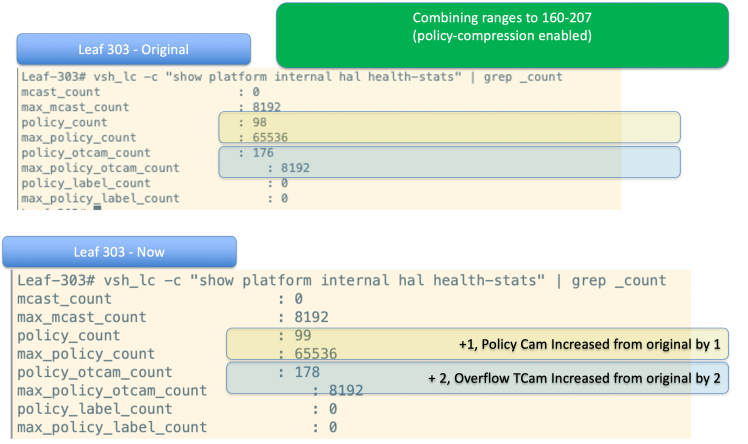
Ofcourse in this simplistic example it’s very easy to spot that the port ranges are overlapping.  In a real ADM output there will be tons of port ranges defined, and it will be hard to spot.  Making a contract based out of this and putting the 3 ranges exactly as they are in the contract we see CAM utilization increase by 3 on Policy CAM and by 10 on Overflow TCAM

Combining the ranges for 1 port range of  tcp 160-207  we notice that the Policy CAM has just increased by 1 and the Overflow TCAM has just increased by 2.   That’s a significant improvement.   It may look like very little in this 2 EPG simple topology, but in a real application with multiple tiers and multiple meshed contracts, with multiple consumers and multiple providers that extra utilization can multiply quickly. 

Must Read Documents:
Everything you want to know about ACI Contracts 
Forwarding Scale Profiles
Scalability Guide for APIC 5.1.1 release

Summary Of Commands Used in this article:

moquery -c fvCtx | grep SM-VRF -A 10     # on APIC, find out scope for VRF

moquery -c fvEPg | grep L30 -B 5 -A 8     # on APIC, find out pcTag for EPG

show zoning-rule scope 2588673     #  on Leaf, use VRF scope to see rules

show zoning-rule src-epg 49153 dst-epg 32770     #  on Leaf, to see rules/filters between a pair of EPGs

vsh_lc -c "show system internal aclqos zoning 4175”     #  on Leaf, use Rule ID  to see hw_index

show zoning-filter filter implarp     #  on Leaf,  to see details of Filter

show system internal policy-mgr stats | grep 2588673     #  on Leaf,  to see hits on rules

show endpoint vrf SM-TestTenant:SM-VRF     #  on Leaf,  to see if endpoint exists on a VRF

moquery -c fvLEpP -f 'fv.LEpP.polInstrumented=="yes"' | grep -A 12 -B 5  L303     # on Leaf, to see if endpoint exist on EPG

vsh_lc -c "show platform internal hal health-stats" | grep _count # on Leaf To see Policy CAM and Overflow TCAM usage

vsh_lc -c "show platform internal hal policy stats region all" # on Leaf to show Regions and Hash Entries

vsh_lc –c “show platform internal hal l3 routingthresholds”     # show LPM Memory related thresholds